Useful Query Patterns
Here we'll lay out some useful patterns frequently encountered in analytical workflows
Cohort Analysis
Often we want to build cohort analyses - facts about users or entities that we join back to users for timeseries or comparative analysis. Here we'll do a quick user_facts table of first purchase, and then an analysis of purchases by month based upon user first purchase month.
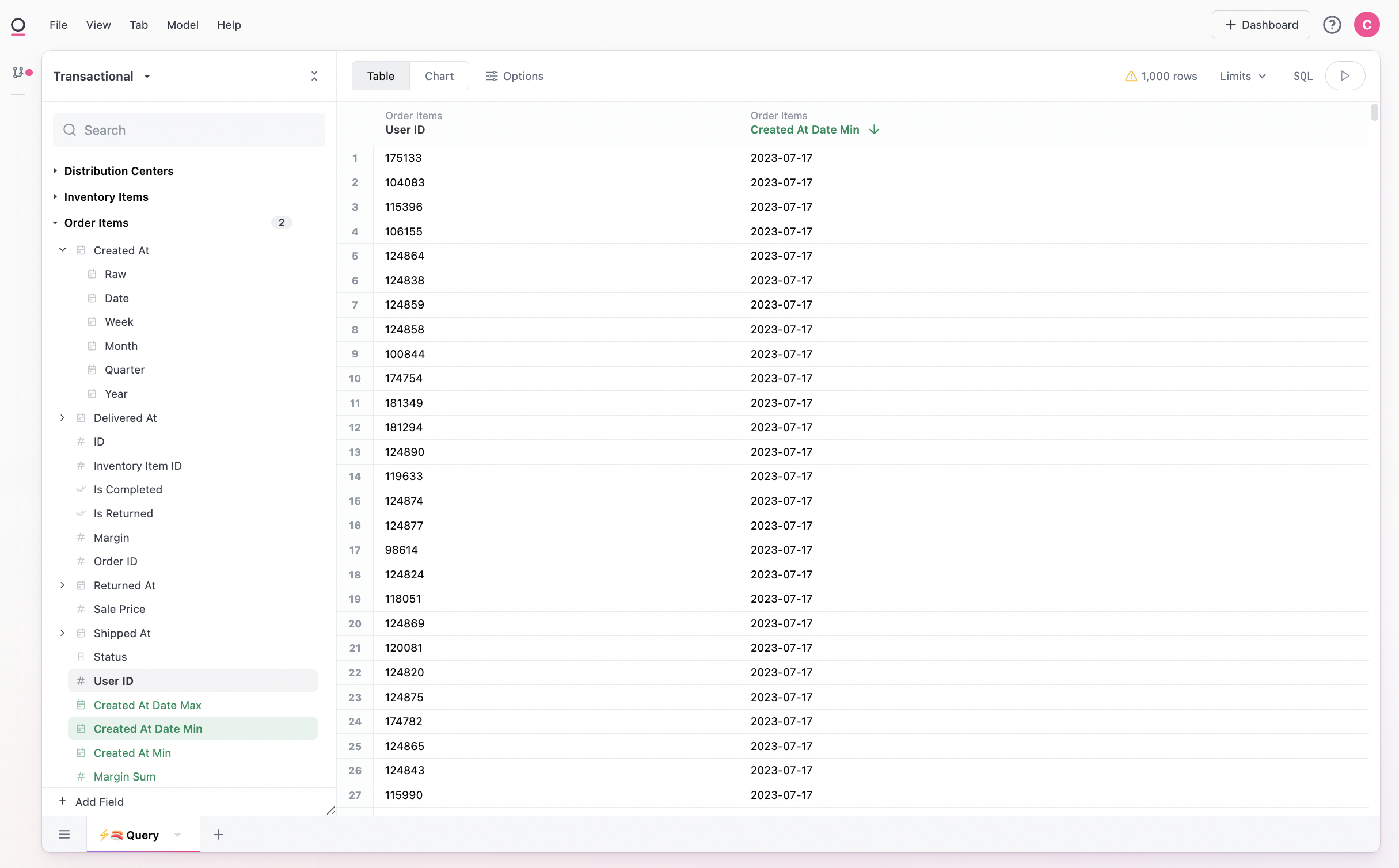
First we'll build our fact table, here user_id and min_created_at from the transactions table, essentially a table of every user and their first purchase:
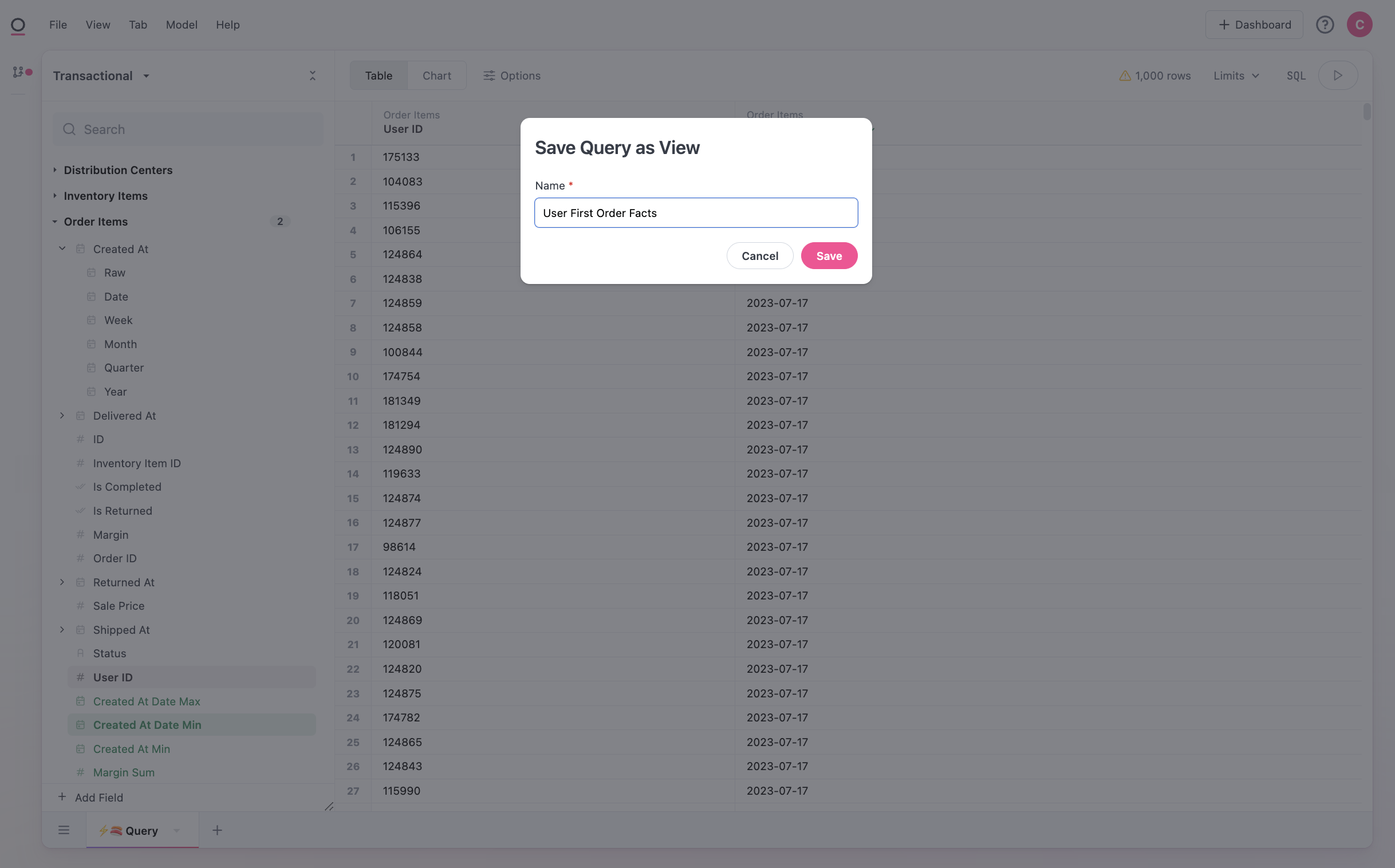
Using the menu in the header, we can select Model > Save Query as View and name our fact table for use in the workbook:
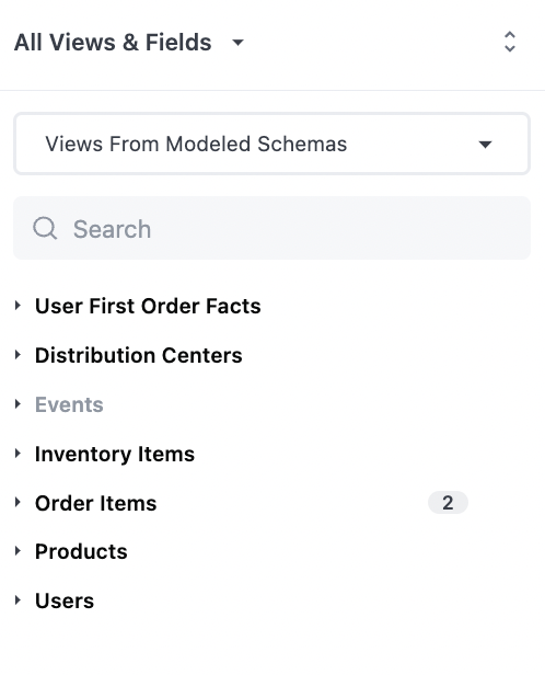
To start querying with our fact table, we can navigate to 'All Views and Fields' in the topic selector. We'll solve the problem later of adding this to our topic:
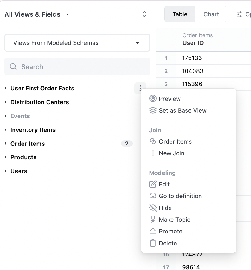
We'll want to confirm that Omni guessed our join properly, by looking at the available joins on our new fact table:
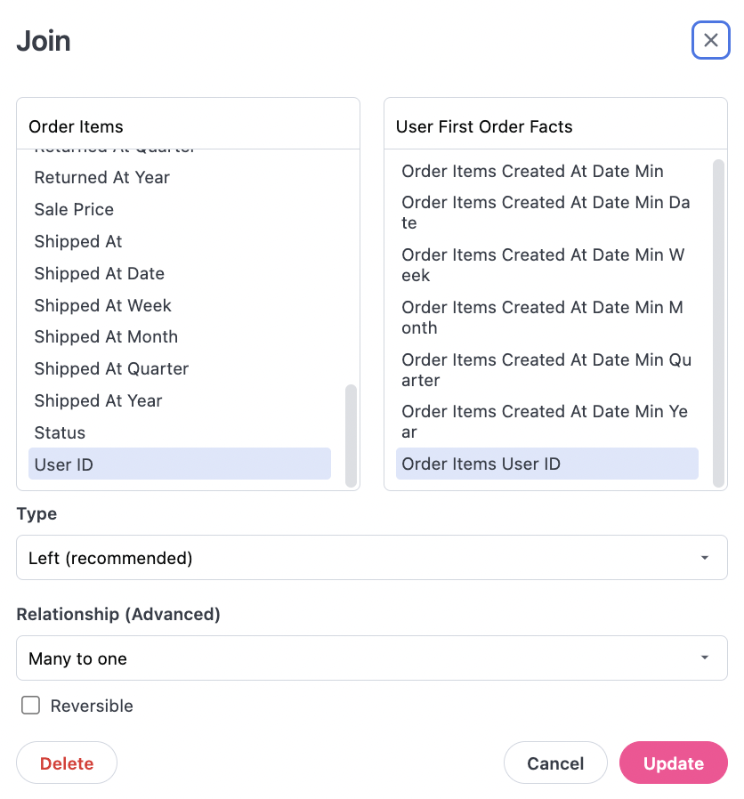
The join modal shows our view will be joined back to orders user user_id, so is doing what we want:
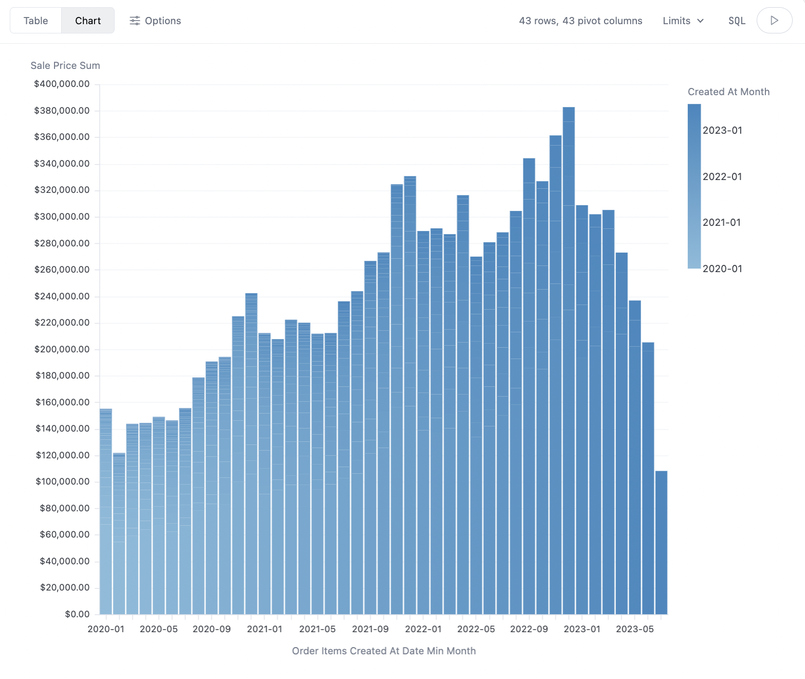
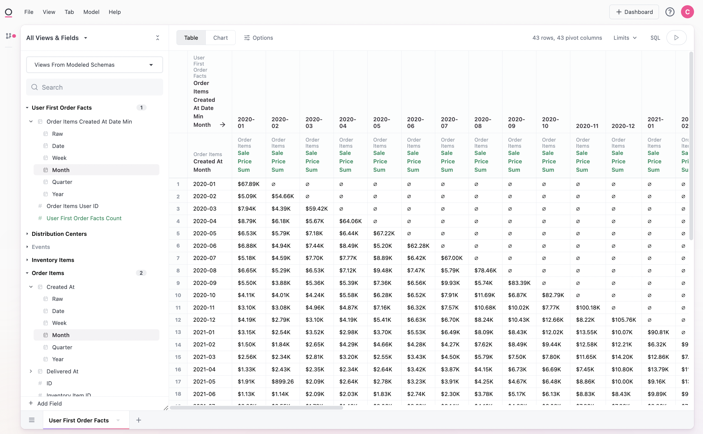
From there we simply need to query across orders and our new fact table (make sure to set the base view as order items here):
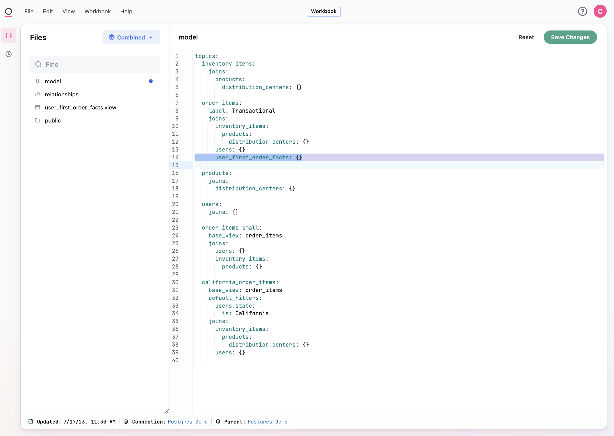
We may want to add this fact table into our topic for easier curation and sharing. We can start by viewing the workbook model in the left nav:
Using the {}, we can enter the workbook model and add our fact table to the order_items topic:
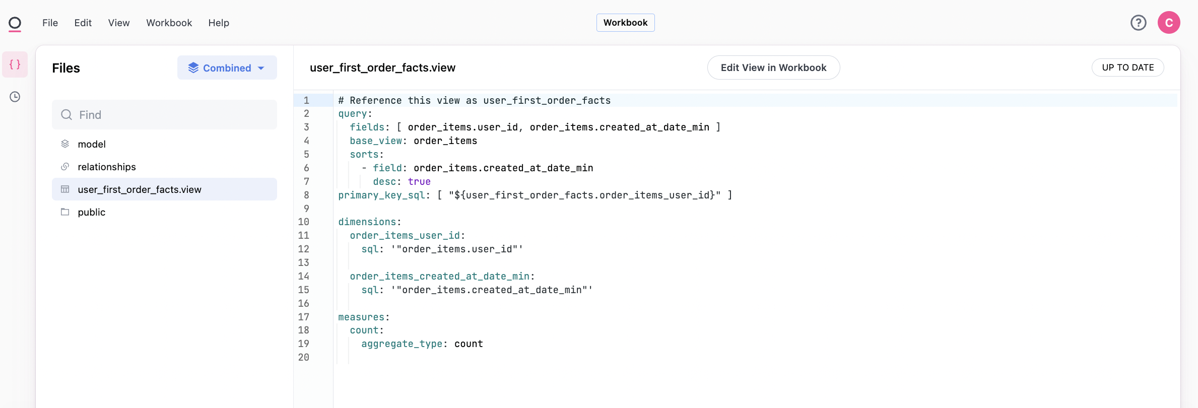
We can take a quick look at the fact table model as well:
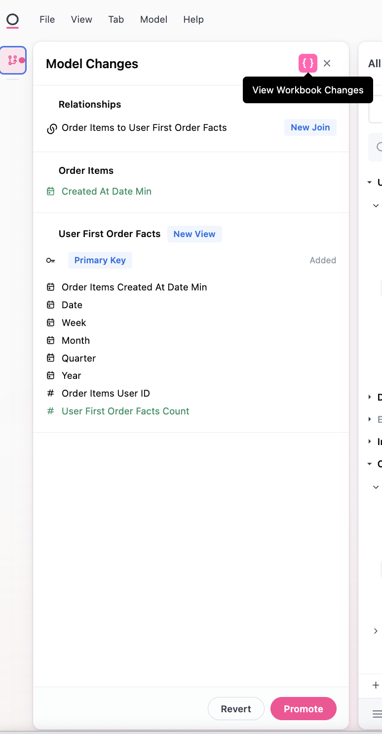
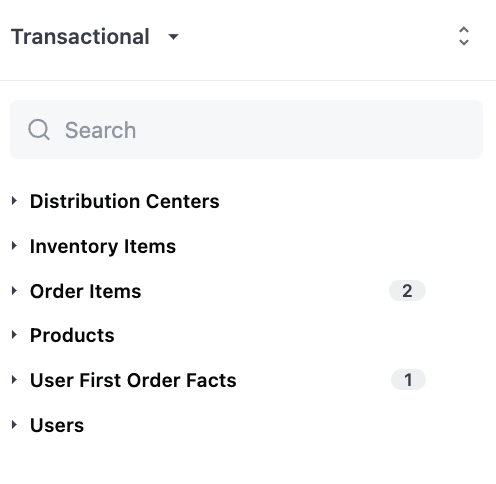
We can confirm the join worked correctly by navigating back to the transactions / order_items topic:
We can then also optionally promote down our fact table into the Shared data model for all analyses, or we could simply leave it in our workbook for this analysis.
Some Extensions to Cohorting
Often we want to go a bit further than time vs time, and, for example, look at periods since vs time. Let's take a quick look at how to do that.
First we'll want to create a time_since field. Here we'll do months since sign-up using 30 day periods. There's lots of additional nuance that could be applied. Postgres has somewhat clunky time diffs, but here we subtract order date from our fact table first order date, and then divide by 30 to get months (EXTRACT(DAY FROM ${order_items.created_at[date]} - ${user_first_order_facts.order_items_created_at_date_min[date]}) and FLOOR(EXTRACT(DAY FROM ${order_items.created_at[date]} - ${user_first_order_facts.order_items_created_at_date_min[date]}) / 30)). There are many ways to tune this calculation differently:
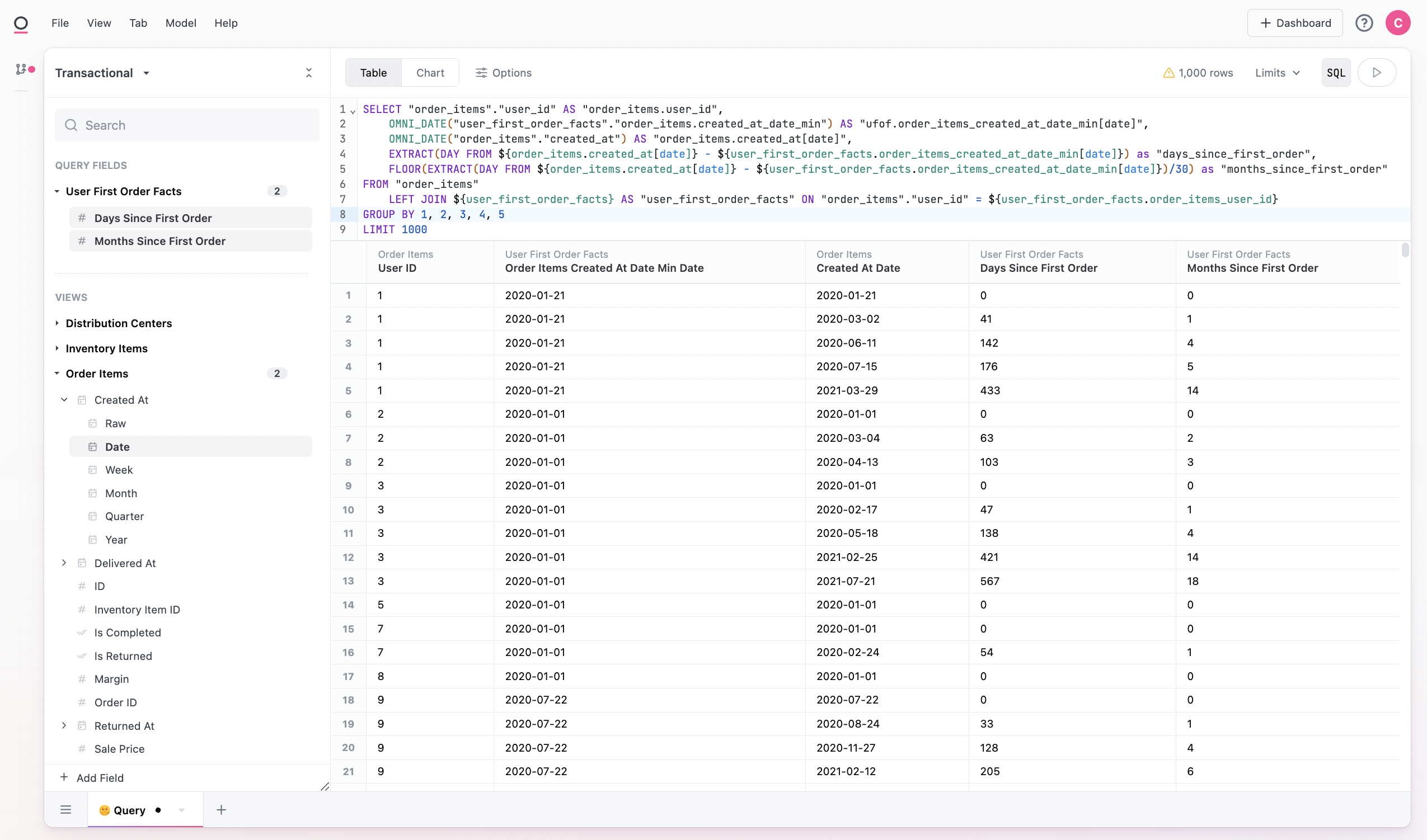
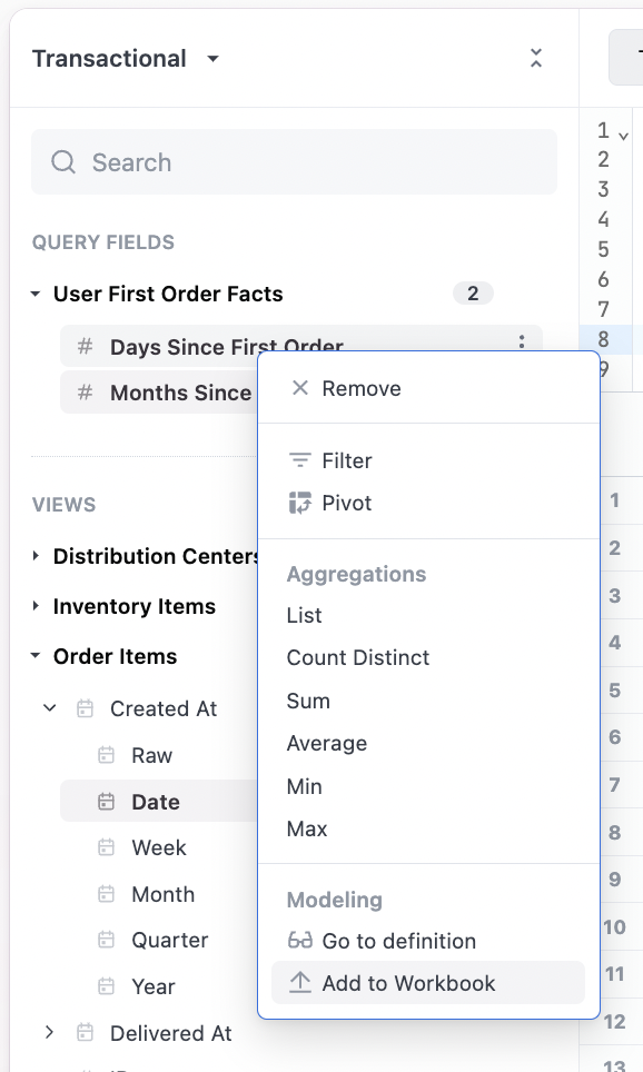
From there, we can add the fields to our workbook. Note these fields were built from the SQL block, but also could have been done via the "Add Field" at the bottom of the field picker or from the workbook model IDE:
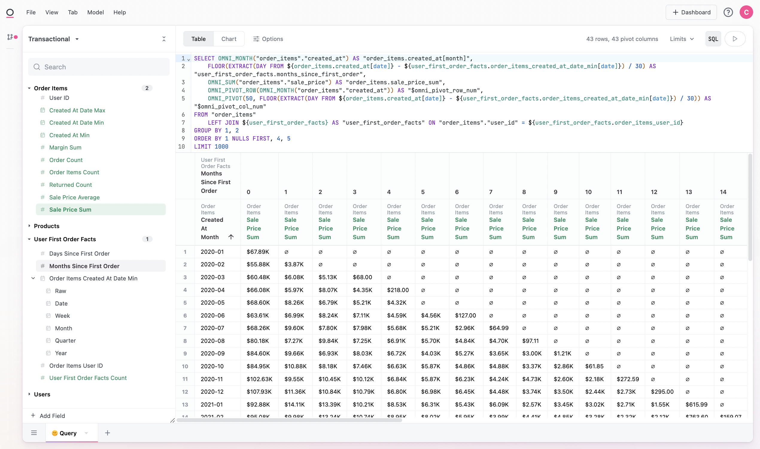
We now have our rebased cohort with periods since instead of the raw date (ie inverted the matrix):
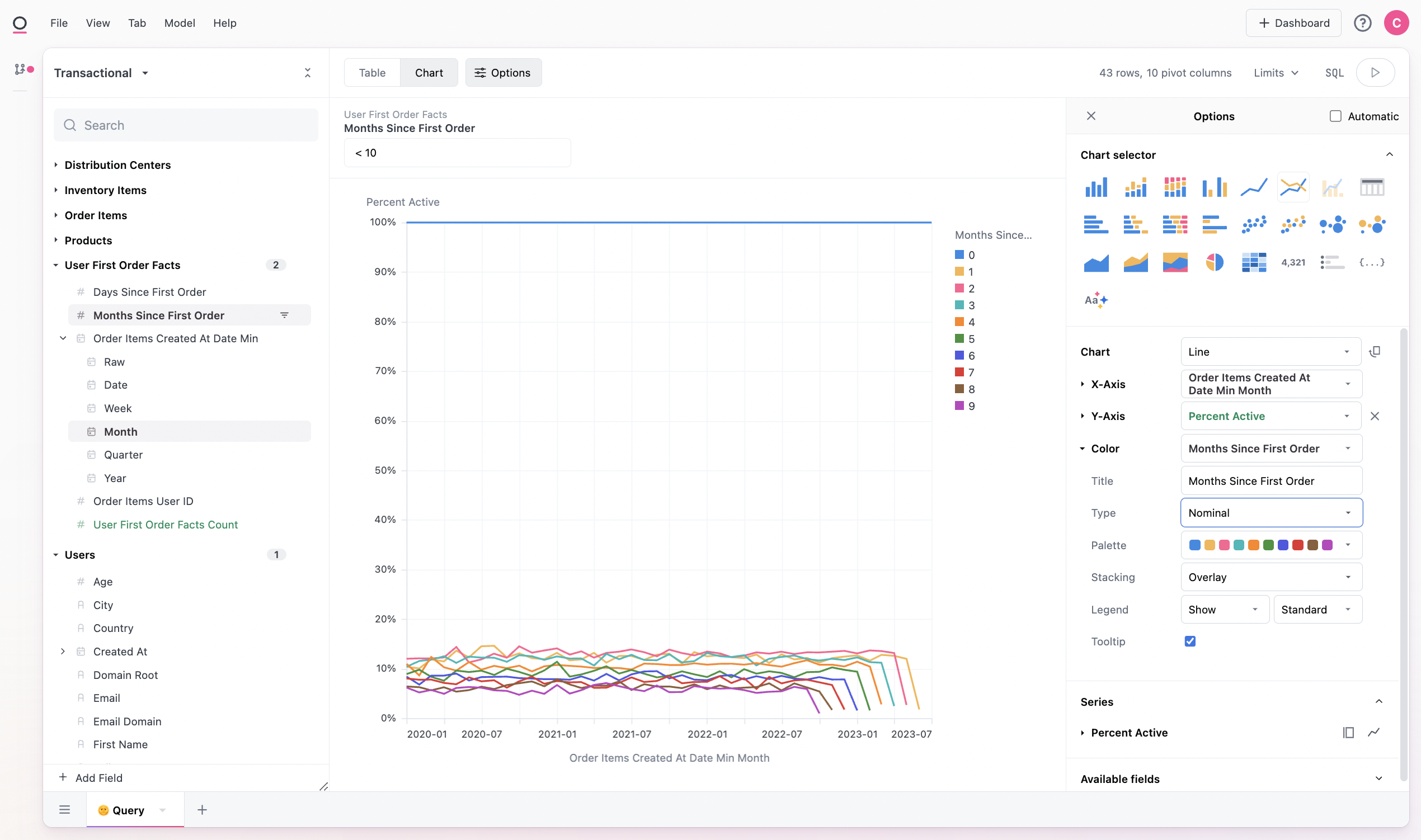
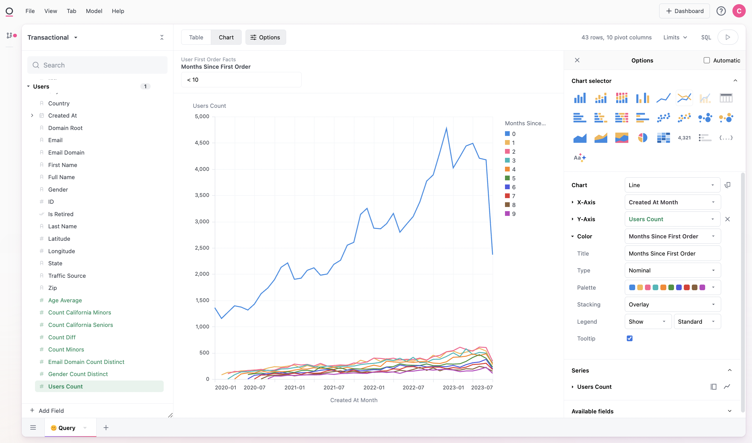
We can also visualize this data, note we add to change the months since field to be a nominal rather than quantitative field for better viewing:
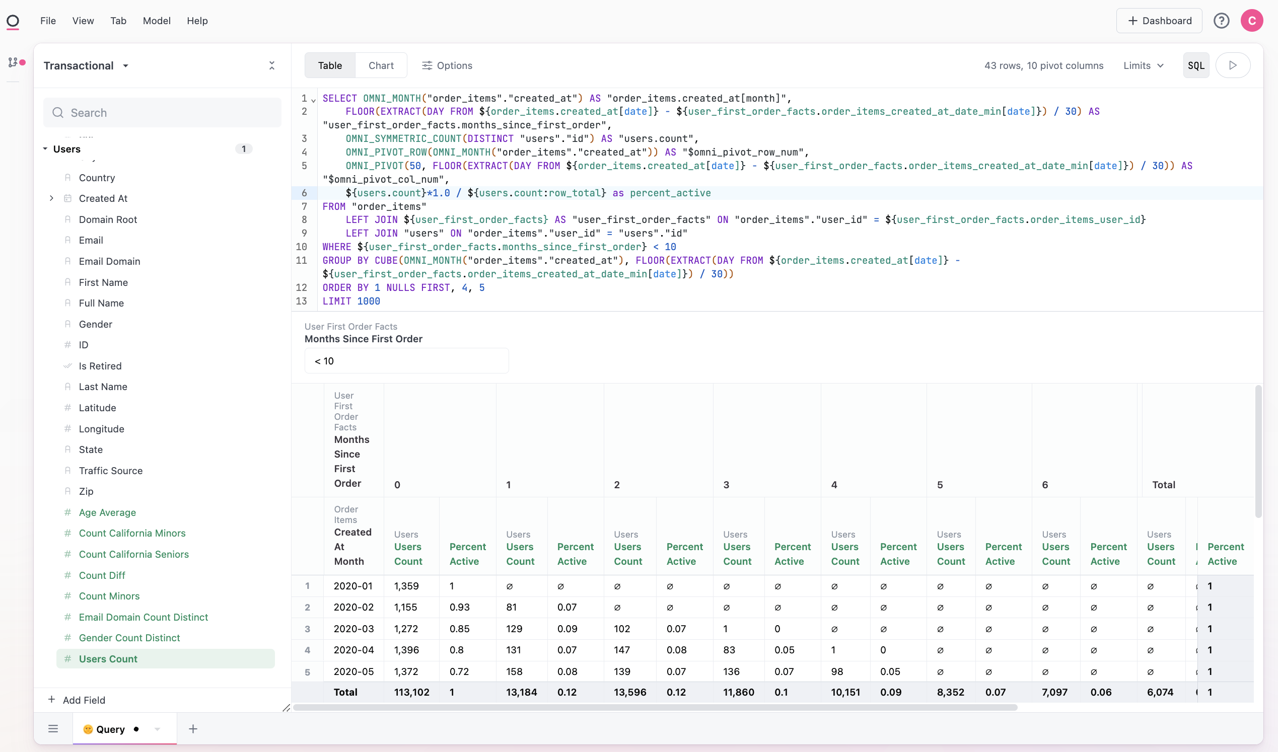
It may also make sense to rebase our measure from a count to a percent active. If we add row and column totals to our query, we can then use these values in our calculation. Here we divide each count cell by the row total, for a percent of the row that is active in a given period (${users.count}*1.0 / ${users.count:row_total}). Note we also add the *1.0 to avoid issues with integer math in SQL:
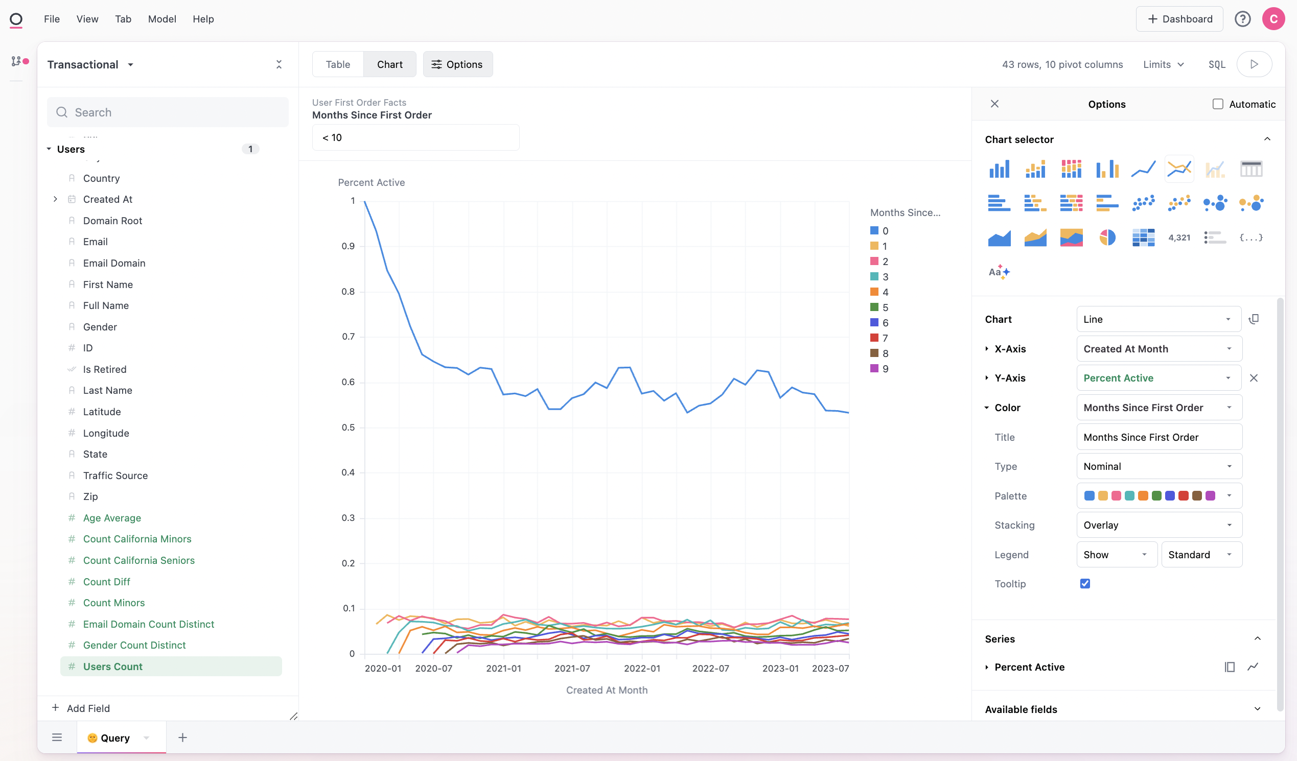
From there we can visual our rebased percentage by swapping the Y-axis in our visualization. Here we look at sales contribution by user age, where we are starting to build a nice tail of long-time users:
Or we could use user sign-up date and look at retention, which looks pretty stable: